
AI & INFRASTRUCTURE
More than you ever wanted to know about Engrams in DeepSeek 4.1
A deep dive into DeepSeek V4.1 Flash’s Engram memory: lookup mechanics, token deadlines, latency tables, SSD experiments and remote RAM over Thunderbolt and Ethernet.
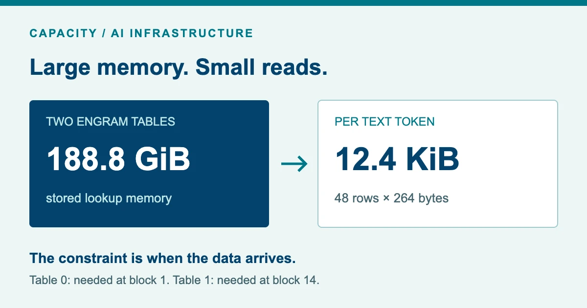
DeepSeek V4.1 Flash ships with 188.8 GiB of n-gram lookup tables. That’s before expert weights, attention caches or anything else the inference engine needs. So does all of it have to sit in RAM—or can an SSD, or even another machine, serve it fast enough?
Each token reads just 48 of those rows: 12.4 KiB. The catch is timing. The first 24 rows are needed after a single layer of compute—about 0.6 ms at 40 tokens/s—and they’re scattered across a 94 GiB file. I worked through the timing and measured the storage I had at hand: an internal and an external SSD on an M5 Ultra, and a second machine’s RAM over Thunderbolt and gigabit Ethernet.
Short answer: give Table 0 the fastest path you have. It’s needed at block 1, while Table 1 can wait until block 14. A decent NVMe drive keeps up to roughly 40–60 tokens/s, and a late read costs a few percent rather than a collapse. Remote RAM over Thunderbolt is faster still, as long as the engine batches the rows into one request. On macOS, DwarfStar currently reads both tables before computing anything, so the read time adds to every token. And don’t quantise the tables harder to save disk: on an SSD a smaller row reads no faster, so the quality you give up buys nothing.
What’s measured and what’s modelled
- Measured: per-row SSD latencies (Python harness, macOS, M5 Ultra, 25 October 2026) and remote-RAM batch round trips (a small C daemon over TCP). I did not run DwarfStar end to end.
- Derived: SSD table-fetch times, calculated as six times the per-row median.
- Modelled: every deadline and the heatmap. They describe DwarfStar’s asynchronous reader at the commit linked at the end, where four reader threads overlap the reads with computation, for a single decode stream. Above 100 tokens/s they are sensitivity analysis.
Terms used in this article
- Token
- The unit a language model reads and writes: a word, part of a word or a punctuation mark, stored as an integer ID.
- n-gram
- A run of n consecutive tokens. Here: the last two, three or four tokens up to the current one.
- Engram
- DeepSeek’s name for a learned n-gram memory. Hashes of recent n-grams pick rows from large tables, and the model mixes those rows into its working state. Trained with the model, not filled at run time.
- Block (layer)
- One step of the model’s stack: attention plus a feed-forward network. V4.1 Flash has 40, numbered 0–39.
- Working state / residual
- The vectors that carry each token through the stack. Every block reads them and adds its result back. V4.1 keeps four parallel streams of this state.
- Hash head
- One of eight independent hash functions per n-gram length. Each produces one row address, so collisions in one head are evened out by the others.
- Row read / table fetch / network batch
- A row read returns one 264-byte row. A table fetch is the 24 rows one block needs. A network batch is one message carrying several row requests. Their latencies can’t be compared directly.
- Mixture of experts (MoE)
- A feed-forward network split into many “experts”, of which only a few run for each token. The expert weights are large, which is why they are sometimes streamed from disk.
- Decode / prefill
- Decode generates one token per step and is what this article times. Prefill processes the whole prompt in one go.
- Speculative decoding
- A small draft model guesses several tokens ahead; the large model checks them in one verification pass.
- p50, p99, p99.9
- Percentiles: half of all reads were faster than p50, 99% faster than p99, 99.9% faster than p99.9.
- IOPS
- Input/output operations per second: how many separate reads a drive completes.
- RDMA
- Remote direct memory access: a network reads another machine’s RAM without involving its CPU. Not used in these tests.
- Quantisation
- Storing values with fewer bits. These tables use 8-bit values with one shared scale per 32 values; a 4-bit version would halve the size but round every value more coarsely.
- KiB / GiB vs KB / GB
- Binary units (1 KiB = 1,024 bytes) versus decimal ones (1 KB = 1,000 bytes). 12.4 KiB is 12,672 bytes.
1. Where Engram sits in the model
V4.1 Flash is a stack of 40 blocks—model layers, nothing to do with SSD blocks. In each one, attention pulls in context from earlier tokens and a mixture of experts transforms the result; both are added back to the working state. Engram adds a third contribution, but only in two blocks, just before attention.
Inside a block
- Receive the working state from the previous block.
- Blocks 1 and 14 only: add the gated Engram value.
- Mix the four streams, normalise, run attention.
- Add the attention result back.
- Mix and normalise again, run the mixture of experts.
- Add that result back and hand the state on.
Inside one Engram lookup
- 4 tokenscurrent + 3 before, compressed IDs
- 3 suffixes × 8 hash headslast 2, 3 and 4 tokens
- 24 rows × 264 Bfetched from RAM, SSD or network
- 6,144 values8-bit, one scale per 32
- 4 keys + 1 value5,120 wide each
- gate × valueadded to each of the 4 streams
The lookup works on token IDs, not text. The engine maps the current token and the three before it into a compressed vocabulary, so some spelling variants share an ID. It hashes the last two, three and four tokens with eight hash heads each: 24 row addresses per table, 48 per token. Each row holds 256 eight-bit values and eight one-byte scales, 264 bytes in all.
| Item | Value |
|---|---|
| Blocks in the model | 40, numbered 0–39 |
| Blocks that use the tables | 1 (Table 0) and 14 (Table 1) |
| n-gram sizes hashed | 2, 3 and 4 tokens |
| Rows per token per table | 24 (3 sizes × 8 hash heads) |
| Row size | 264 B (256 values + 8 one-byte scales) |
| Read per text token | 48 × 264 = 12,672 B ≈ 12.4 KiB |
| Tables on disk | 188.8 GiB total |
| Lookback kept per inference request | Last 3 compressed token IDs |
The rows become four keys—one per working stream—and one shared value. Each stream compares its state with its key, and the score becomes a gate between zero and one. It’s learned memory inside the forward pass, closer to an embedding table than to retrieval-augmented generation; nothing is inserted into the prompt. Image-placeholder positions are masked, and the speculative decoder’s draft model doesn’t use Engram at all.
2. One token, from lookup keys to output
The row addresses depend only on token IDs, so the CPU can compute them and start reading before the GPU reaches block 1. With the asynchronous reader, block 0 hides the Table 0 reads, and blocks 1 to 13 hide Table 1. macOS works differently—open the last drill-down or see chapter 3.
- Table 0
- 1 block
- Table 1
- 13 blocks
- Blocks 15–39
- no Engram I/O
The four reader chains
Each worker reads six Table 0 rows (dark), then six Table 1 rows (light). There is no barrier between the tables, so worker 3’s slow read delays Table 0 while the others already work on Table 1. Illustrative timings.
Step by step
- The CPU hashes the token and its lookback; four reader threads start on Table 0. The token is embedded.
- Block 0 runs attention and experts while the reads continue.
- Block 1 waits for Table 0 if needed, projects, gates and adds, then runs as usual.
- Blocks 2–13 run while the same readers fetch Table 1.
- Block 14 consumes Table 1 the same way: the second and last injection.
- Blocks 15–39, the output layer and sampling pick the next token. The consumed token joins the three-token history.
The macOS path at this commit
No overlap reader: both tables are read with 16 workers before the token is embedded, and the GPU waits for all of it.
3. The timing model
The asynchronous token path uses TOKEN_READERS = 4. Each worker reads six rows per table in sequence, so the per-row budget is the table’s window divided by six. At 40 tokens/s Table 0 has about 625 µs, roughly 104 µs per row. Under four-reader load the median row read took 68 µs on the internal SSD and 99 µs on the external one—both inside the budget. At 100 tokens/s the budget drops to 42 µs and both miss.
| Baseline | Token timems | Table 0 windowms · 1 block | Table 1 windowms · 13 blocks | Table 0 row budgetµs | Table 1 row budgetµs | Payloadreads/s · MB/s |
|---|---|---|---|---|---|---|
| 15 t/s | 66.67 | 1.667 | 21.67 | 278 | 3,611 | 7200.19 |
| 20 t/s | 50.00 | 1.250 | 16.25 | 208 | 2,708 | 9600.25 |
| 30 t/s | 33.33 | 0.833 | 10.83 | 139 | 1,806 | 1,4400.38 |
| 40 t/s | 25.00 | 0.625 | 8.13 | 104 | 1,354 | 1,9200.51 |
| 60 t/s | 16.67 | 0.417 | 5.42 | 69.4 | 903 | 2,8800.76 |
| 70 t/s | 14.29 | 0.357 | 4.64 | 59.5 | 774 | 3,3600.89 |
| 100 t/s | 10.00 | 0.250 | 3.25 | 41.7 | 542 | 4,8001.27 |
| Above 100 t/s: single-stream sensitivity analysis | ||||||
| 300 t/s | 3.33 | 0.083 | 1.08 | 13.9 | 181 | 14,4003.80 |
| 600 t/s | 1.67 | 0.042 | 0.54 | 6.9 | 90.3 | 28,8007.60 |
With those medians, the internal drive keeps up to about 61 tokens/s and the external one to about 42. That’s arithmetic on a median; the tail is in chapter 4.
A late table costs its overshoot
Missing a window isn’t a cliff. A late fetch adds only the time by which it overshoots; the blocks already computed stay computed.
Thunderbolt batch · 0.095 ms fetchno stall
External SSD, 4 × 6 reads · 0.59 ms fetch+0.34 ms stall
At 100 tokens/s that overshoot is 0.34 ms on a 10 ms token: 3.4% more time, about 96.7 tokens/s. The same 100 µs overshoot costs 0.4% of a 25 ms token and 6% of a 1.67 ms one—the faster the GPU, the less time storage has to hide. At a hypothetical 600 tokens/s even Table 1 misses with 0.59 ms fetches (442 tokens/s), and a 2.4 ms fetch, roughly one reader working through all 24 rows, leaves about 170.
The formula and its limits
w₀ = W / 40
w₁ = 13W / 40

extra = max(0, f₀ − w₀)
      + max(0, f₁ − w₁)

T = W + extra  (ms)
slowdown = extra / W
tokens/s = 1000 / T
W is the token time without Engram stalls, f₀ and f₁ the two fetch times, and every block counts as W/40. The formula is exact when Table 0 misses, because block 14 moves back by the same stall, and slightly pessimistic when Table 0 arrives early. Real workers overlap the two tables, early Table 1 reads can queue behind Table 0, and embedding, sampling, the output head and CPU–GPU synchronisation take part of W. Treat it as a planning tool until you have a trace.
264 bytes in, kilobytes off the flash
The logical payload is tiny: 1.27 MB/s at 100 tokens/s. The drive moves more. If every row read pulls a 4 KiB page, 600 tokens/s means 28,800 reads/s and about 118 MB/s; with 16 KiB pages it’s about 472 MB/s. Either way, for one stream random-read latency matters and an SSD’s sequential GB/s rating says little.
macOS works differently at this commit. Non-Apple builds create the asynchronous reader and overlap its four workers with computation, unless DS4_DISABLE_V41_ENGRAM_OVERLAP is set. On macOS the reader is never created, so the token step reads Table 0 and then Table 1 through ds4_engram_read_batch before embedding and block 0. That batch reader uses 16 workers from eight rows up on Apple platforms (from 256 rows elsewhere, so large prefill batches use 16 too).
Nothing hides those reads: if F is the time for both batches, a token takes T = W + F. The windows, the heatmap and the four-reader SSD estimates don’t apply, so F has to be measured on its own.
4. Inside the SSD experiments
I ran the disk tests on an Apple M5 Ultra with 256 GiB RAM under macOS, using Python’s os.pread with F_NOCACHE to keep the file cache out. The internal SSD read a 2 GiB zero-filled scratch file; the external Samsung 4 TB volume read an actual 94.4 GiB Engram table. One reader, then four, 264 bytes per read, about four seconds each. The harness times single reads, never a whole 24-row lookup—hence the derived 6 × 68 µs = 0.41 ms and 6 × 98.6 µs = 0.59 ms per table.
- p50
- p99
- p99.9
- max
- ATable 0 row budget at 40 t/s (104 µs)
- BTable 0 row budget at 100 t/s (42 µs)
One read in a thousand takes 2 ms
On the external drive with four readers, the median row read was 98.6 µs, but the p99.9 was 2.05 ms and the slowest read took 36.8 ms. One read like that stalls its whole chain, and the fetch waits for the slowest of the four chains. Using the 121.4 µs mean instead of the median gives 0.73 ms per table and 4.8% extra token time at 100 tokens/s—and even that is a floor, because the slowest of four chains takes at least six times the mean on average.
All measured values
| Device / readers | Row p50 (µs) | Mean (µs) | p99 (µs) | p99.9 (µs) | Maximum (µs) | IOPS |
|---|---|---|---|---|---|---|
| Internal · 1 reader | 64.3 | 61.0 | 90.5 | 122.4 | 1,097 | 16,280 |
| Internal · 4 readers | 68.1 | 64.1 | 109.0 | 157.5 | 1,199 | 61,849 |
| External · 1 reader | 98.2 | 100.6 | 217.4 | 294.3 | 4,734 | 9,883 |
| External · 4 readers | 98.6 | 121.4 | 170.9 | 2,048.1 | 36,790 | 32,708 |
Smaller quants buy space, not speed
Fewer bits per value look like an easy win. A 4-bit row would be 136 bytes instead of 264, and both tables would shrink from 188.8 to about 97 GiB. But the SSD doesn’t care: on the internal drive a 264-byte read had a 64.25 µs median and a 4 KiB read 68.38 µs; on the external drive 98.17 and 99.79 µs. Fifteen times the data barely moved the access time, because the drive fetches a whole page either way.
| Row format | Rowbytes | One tableGiB | Both tablesGiB |
|---|---|---|---|
| 4-bit + scaleshypothetical | 136 | 48.6 | 97.3 |
| 8-bit + scalesas shipped here | 264 | 94.4 | 188.8 |
| 16-bithypothetical | 512 | 183.1 | 366.2 |
So a harder quant only pays if it changes where a table lives—if a 4-bit Table 0 at about 49 GiB fits in RAM where the 8-bit one at 94 GiB doesn’t. On the same SSD it saves no time and costs quality: every lookup, at every token, gets coarser values. I haven’t measured how much a 4-bit Engram table hurts output, but it’s a trade with nothing on the other side. If disk space is the constraint, buy a bigger SSD. The same logic runs the other way: a 512-byte 16-bit row is still far smaller than a 4 KiB page, so keeping more precision on SSD would cost disk space, not read time.
More readers, more drives?
A second harness ran 8 to 48 concurrent readers on each drive and split across both. With eight readers, splitting four per drive cut the per-read p99 from about 265 µs to about 150 µs, while the median got slightly worse (86 → 93 µs). At 24 readers the ranking reshuffled between repeat runs, and at 48 the median rose to about 235 µs: more outstanding reads mostly mean more queueing. A second drive may help the tail and can keep Engram away from expert-weight streaming. This was a two-drive split, though, and a RAID 0 array might behave differently.
All ten reader configurations
| Layout / readers | Per-read p50 (µs) | Per-read p99 (µs) | Harness-round p50 (µs) | Harness-round p99 (µs) |
|---|---|---|---|---|
| 8 readers · internal only | 86.1 | 264.8 | 194.8 | 400.9 |
| 8 readers · split 4 + 4 | 93.4 | 149.6 | 203.6 | 312.3 |
| 8 readers · external only | 103.5 | 171.0 | 226.7 | 346.8 |
| 12 readers · internal only | 88.6 | 185.6 | 247.6 | 504.4 |
| 12 readers · external only | 106.8 | 200.8 | 288.4 | 506.3 |
| 12 readers · split 6 + 6 | 97.7 | 189.8 | 262.5 | 508.8 |
| 24 readers · internal only | 140.6 | 328.2 | 483.2 | 892.6 |
| 24 readers · external only | 119.4 | 314.3 | 464.3 | 936.5 |
| 24 readers · split 12 + 12 | 145.7 | 361.0 | 487.3 | 1,102.4 |
| 48 readers · split 24 + 24 | 235.3 | 595.0 | 974.4 | 1,590.4 |
Short runs, different file sizes, sustained load and hosts that weren’t fully idle limit how far this generalises, and the same drive may behave differently with another OS or I/O stack. The next useful measurement is a real token-paced fetch alongside the actual competing workload.
5. Remote RAM, Thunderbolt and Ethernet
Memory disaggregation sounds grand; here it just means putting a table in another machine’s RAM and asking it for rows. My test used a small C daemon over TCP, serving a synthetic 4 GiB buffer with one request in flight—transport plus service time, outside any inference engine.
- ATable 0 window at 100 t/s (0.25 ms)
- BTable 0 window at 40 t/s (0.625 ms)
Over a 20 Gb/s Thunderbolt link (TCP, no RDMA), one 24-row batch took 92–99 µs, with a p99 of 139–158 µs; a 48-row batch for both tables took about 100 µs. If each worker instead made six round trips of about 90 µs, a table would take about 0.54 ms—roughly what the external SSD manages. The win comes from one message per table, and the engine has to implement that. With it, Table 0 makes its window up to about 250–270 tokens/s in the model.
Gigabit Ethernet and UDP
Over wired 1 Gb Ethernet, a 24-row batch took 0.60–0.70 ms with TCP and TCP_NODELAY. Serialising 6,336 bytes takes only about 51 µs, and a bulk transfer on the same path reached 117 MB/s, so the time goes into the round trip itself: link, NIC, kernel and service. Energy-efficient Ethernet settings, jumbo frames or 2.5/10 Gb Ethernet might help; I haven’t measured them.
I expected UDP to be faster. It wasn’t: about 0.85 ms against 0.71 ms for TCP in a back-to-back check, with the 6.3 KB reply split into about five IP fragments.
The memory still has to exist somewhere
The donor has to keep the whole table resident, plus room for the OS and the service: 128 GB is about 119.2 GiB, which leaves about 24.8 GiB once a 94.4 GiB table is loaded. You also need access control, matching table versions, timeouts, monitoring and a fallback for when the peer disappears. Remote RAM swaps a capacity problem for a service dependency—so if Table 0 fits in local RAM, put it there.
6. Nine storage paths, compared
Four of these paths are measured or derived; the rest are estimates and assumptions to see what happens as latency grows. “External SSD” means the drive I tested.
- ATable 0 window at 100 t/s (0.25 ms)
- BTable 0 window at 40 t/s (0.625 ms)
- CTable 1 window at 100 t/s (3.25 ms)
Schedule and evidence for each path
| Storage / link | One-table fetch | Schedule | Evidence |
|---|---|---|---|
| In-memory (same machine) | ≈1 µs | Local gather assumed; schedule not benchmarked | AssumedIllustrative in-memory latency. |
| Remote RAM · Thunderbolt | 92–99 µs | One 24-row TCP batch | MeasuredSynthetic 4 GiB buffer; transport plus service. Heatmap uses 95 µs. |
| Fast local SSD | ≈0.41 ms | 4 parallel readers × 6 sequential rows | Derived6 × 68.1 µs four-reader row p50; 2 GiB zero-filled file. |
| Typical external SSD | ≈0.59 ms | 4 parallel readers × 6 sequential rows | Derived6 × 98.6 µs four-reader row p50; real 94 GiB table. |
| Remote RAM · 1 GbE | 0.60–0.70 ms | One 24-row TCP batch | MeasuredSynthetic 4 GiB buffer. Heatmap uses 0.630 ms. |
| Remote RAM · 100 MbE | ≈1.0 ms | One 24-row batch assumed | EstimatedIllustrative estimate for a slower link. |
| Slower local SSD | 1.5 ms | 4 readers × 6 rows assumed | AssumedIllustrative slower drive. |
| Remote RAM · Wi-Fi | ≈4 ms (2–10 ms) | One 24-row batch assumed | EstimatedIllustrative; wireless latency varies widely. |
| Spinning disk | ≈30 ms | Per-table scenario; reader schedule unspecified | AssumedIllustrative per-table latency. |
What that does to decode speed
The chapter 3 formula, applied to every path at baseline speeds from 25 to 300 tokens/s.
Scroll sideways for all nine paths; the first column stays put.
- No stall
- Some: above 0%, below 30%
- High: 30% or more
| Baselinet/s | Local RAM0.001 msAssumed | Thunderbolt RAM0.095 msMeasured | Fast SSD0.41 msDerived | External SSD0.59 msDerived | 1 GbE RAM0.63 msMeasured | 100 MbE RAM1 msEstimated | Slow SSD1.5 msAssumed | Wi-Fi RAM4 msEstimated | Spinning disk30 msAssumed |
|---|---|---|---|---|---|---|---|---|---|
| 25 | 25no stall | 25no stall | 25no stall | 25no stall | 25no stall | 25no stall | 25+1.3% | 23+7.5% | 12+115% |
| 50 | 50no stall | 50no stall | 50no stall | 50+0.5% | 50+0.7% | 49+2.5% | 48+5.0% | 43+18% | 14+265% |
| 75 | 75no stall | 75no stall | 75+0.6% | 74+1.9% | 73+2.2% | 71+5.0% | 69+8.8% | 59+28% | 15+415% |
| 100 | 100no stall | 100no stall | 98+1.6% | 97+3.4% | 96+3.8% | 93+7.5% | 89+13% | 69+45% | 15+565% |
| Above 100 t/s: single-stream sensitivity analysis | |||||||||
| 125 | 125no stall | 125no stall | 122+2.6% | 119+4.9% | 119+5.4% | 114+10% | 108+16% | 76+65% | 15+715% |
| 150 | 150no stall | 150no stall | 145+3.7% | 141+6.4% | 140+7.0% | 133+13% | 125+20% | 81+85% | 16+865% |
| 175 | 175no stall | 175no stall | 167+4.7% | 162+7.8% | 161+8.5% | 152+15% | 141+24% | 85+105% | 16+1,015% |
| 200 | 200no stall | 200no stall | 189+5.7% | 183+9.3% | 182+10% | 170+18% | 157+28% | 89+125% | 16+1,165% |
| 225 | 225no stall | 225no stall | 211+6.7% | 203+11% | 201+12% | 188+20% | 170+33% | 92+145% | 16+1,315% |
| 250 | 250no stall | 250no stall | 232+7.8% | 223+12% | 221+13% | 204+23% | 179+40% | 94+165% | 16+1,465% |
| 275 | 275no stall | 275+0.1% | 253+8.8% | 242+14% | 239+15% | 220+25% | 186+48% | 96+185% | 16+1,615% |
| 300 | 300no stall | 299+0.4% | 273+9.8% | 260+15% | 258+16% | 235+28% | 194+55% | 98+205% | 16+1,765% |
At 100 tokens/s the internal SSD gives about 98 tokens/s and the external one about 97. A 4 ms Wi-Fi round trip drops it to about 69, because it misses both windows. A constant 1.5 ms fetch fits Table 1’s window up to about 217 tokens/s; the 30 ms spinning disk misses it at every speed. The heatmap holds latency constant—the spread from chapter 4 comes on top.
7. What to build, and what to measure next
- Place the urgent table first. Local RAM if it fits. Otherwise compare a measured SSD path with a properly batched remote-RAM setup. Capacity and sequential throughput are the wrong ranking.
- Protect the read window. Expert streaming, other requests and background I/O all compete for the same drive. A measurement on an idle device says little about a shared production volume.
- Measure the whole wait. Record Table 0 and Table 1 completion times, token stalls and tail percentiles. The slowest of four chains matters more than the median row.
- Test degraded operation. A remote donor can restart, swap or disappear. Decide whether to fall back, retry or reject the request, and measure what the user sees.
- Keep capacity and speed separate. These tables are only one part of model memory. Budget the other weights, attention state, runtime buffers and concurrency headroom too.
- Don’t trade quality for disk space. On an SSD a smaller row reads no faster. Quantise the tables harder only if it moves Table 0 into RAM; otherwise keep the precision.
Prefill, speculation and batches change the workload
Prefill hashes and reads many prompt positions in one wide sweep. A speculative verification pass with k draft tokens covers k+1 positions and requests up to (k+1) × 48 rows; a serving batch multiplies that again. Draft tokens are known before verification, so an engine could prefetch their rows while drafting—an idea I haven’t measured.
The two measurements I’d do next: a token-paced trace of DwarfStar’s asynchronous reader, with expert streaming running alongside, and the synchronous F on a Mac, since that’s the time every token pays there today.
Sources, data and limits
Architecture and reader scheduling refer to DwarfStar at commit ee7e840, an inference engine for DeepSeek V4.1 Flash. See also the model configuration and DwarfStar model card; those two links point to main branches and may change.
The measurements come from my standalone storage harnesses, run on 25 October 2026. You can download the recorded SSD and split-disk measurements at their original precision, with local paths removed; the network samples aren’t included.
Size the system around the workload.
At Capacity, we help teams build private AI systems around their data and operating constraints. Bring us the model, the hardware budget and the response time your users need, and we’ll help turn them into a deployment you can test.
Talk to Andreas hello@capacity.at